OSS Sandpit – Resource / Inventory Module

This article provides a description of the inventory baseline, one module of our Personal OSS Sandpit Project.

As outlined in the diagram below, this incorporates the Inventory solution (by Kuwaiba), the graph database that underpins it as well as its APIs and data query tools. The greyed out sections are to be described in separate articles.

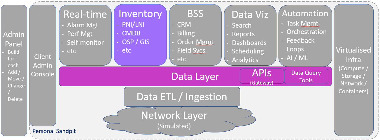
We’ve tackled inventory first as this provides the base data set about resources in the network that other tools rely upon.

As the baseline introduction to the inventory module, we’ll provide a quick introduction to the following use-cases:

• Building Reference Data like data hierarchies, device types, connectivity types, containment, device layouts, templates, flexible data models, etc
• Creating Device Instances including rack views
• Creating Physical Connections between devices
• Creating Logical Connections between devices
• Creating Services and their relationships with resources / inventory
• Creating Outside Plant Views on geo-maps that include buildings, pits, splice cases, cable management, splicing, towers, antenna, end-to-end L1 circuits
• Assigning IP Addresses and subnets with an IPAM tool
• Creating an MPLS network
• Creating an SDH network
• Data import / export / updates via APIs including Service Impact Analysis (SIA)
• Data import / export / updates via a Graph Database Query Language

Reference Data

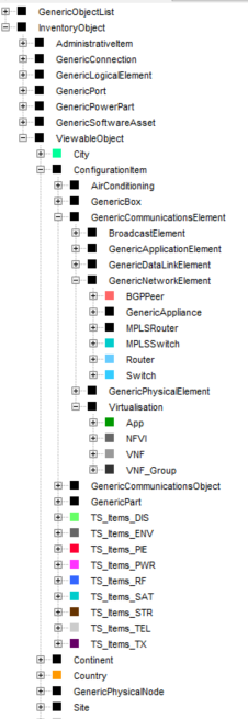
Kuwaiba has a highly flexible and extensible data model. We’ve added many custom data classes (eg device categories like routers, switches, etc) such as those shown below:

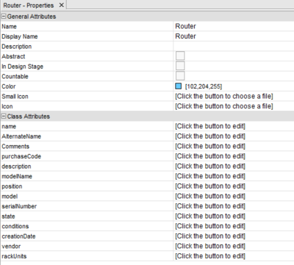
And selectively added custom attributes to each of the classes (such as the Router class below):

Once the classes are created, we then create the Containment model (ie hierarchy of data objects). In our prototype, we’ve developed a custom containment model as follows:

• Country
  • Site
    • System (Network Domain)
      • Rack
        • Equipment and so on.

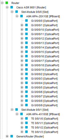
We’ve also created a series of data templates to simplify data entry, such as the Cisco ASR 9001 and Generic Router examples below:

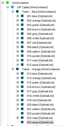
But we can also create templates for other objects, such as cables. The following sample shows a 24 fibre cable with two loose-tubes, each containing 12 fibre strands. (Note that colour-coding on tubes and strands is important for splicing technicians and designers)

Site and Device Instances

Next, we created some sites and devices within the sites, as shown below:

You’ll notice that some devices are placed inside a rack whilst others aren’t. You’ll also notice the naming convention for all devices (eg site – system – type – index, where site = 2052, system = DIS (distribution), type = CD (CD player for messaging) and index = 01 (the first instance of CD player at this site)).

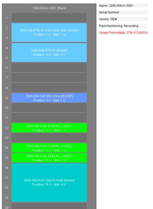
It even allows us to show rack layouts (of equipment positions inside a rack)

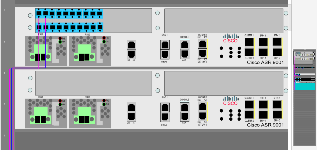
And even patching-level details inside the rack (pink and blue lines represent patch-leads connecting to ports on the Cisco ASR 9001 router in rack position 2):

Physical Connections

Physical connections can take the form of patch-leads or via strands / conductors inside cables.

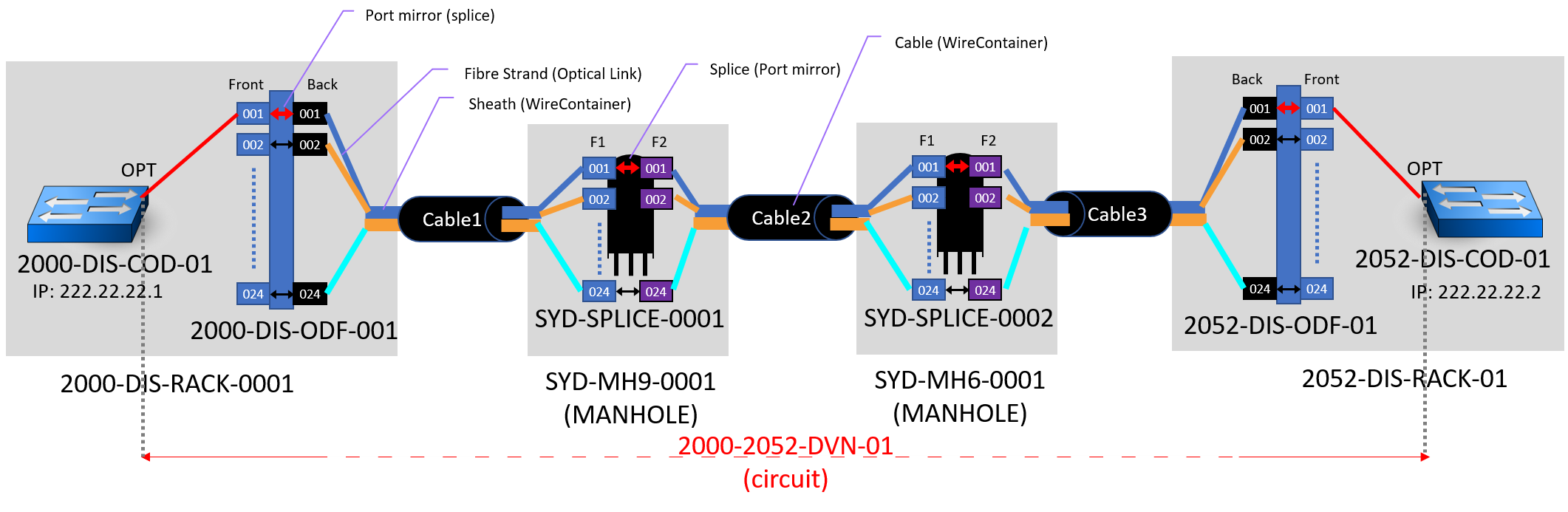
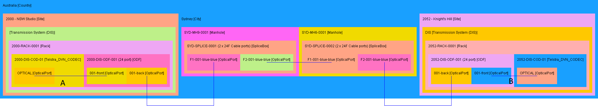
The diagram below represents a stylised optical fibre connection that we’ve created between a CODEC at site 2000 and another CODEC at site 2052. As you’ll also notice, it traverses two patch panels (ODFs – optical distribution frames), two splice joints and three optical fibre cables.

In our inventory tool, the stylised connection above presents as follows, where A and B have been added to indicate the patch-leads from the CODECs to patch-panels (ODFs):

Logical Connections

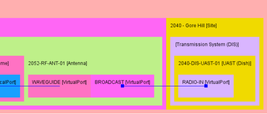
We can also represent logical and virtual connections. In the case below, we show a logical connection from the Waveguide of an antenna, to the broadcast of that signal to a neighbouring site, which then picks up the signal at the UAST (receiver).

Outside Plant Views

Outside plant (OSP) are the cables, joints, manholes, etc that help connect sites and equipment together. In the example below, we see the OSP view of the fibre circuits we described above in “Physical Connections.” If you look closely on the GIS (map overlay) below, you’ll spot sites 2000 and 2052, as well as the cables and splice joints. The lines show the physical route that the cables follow. 

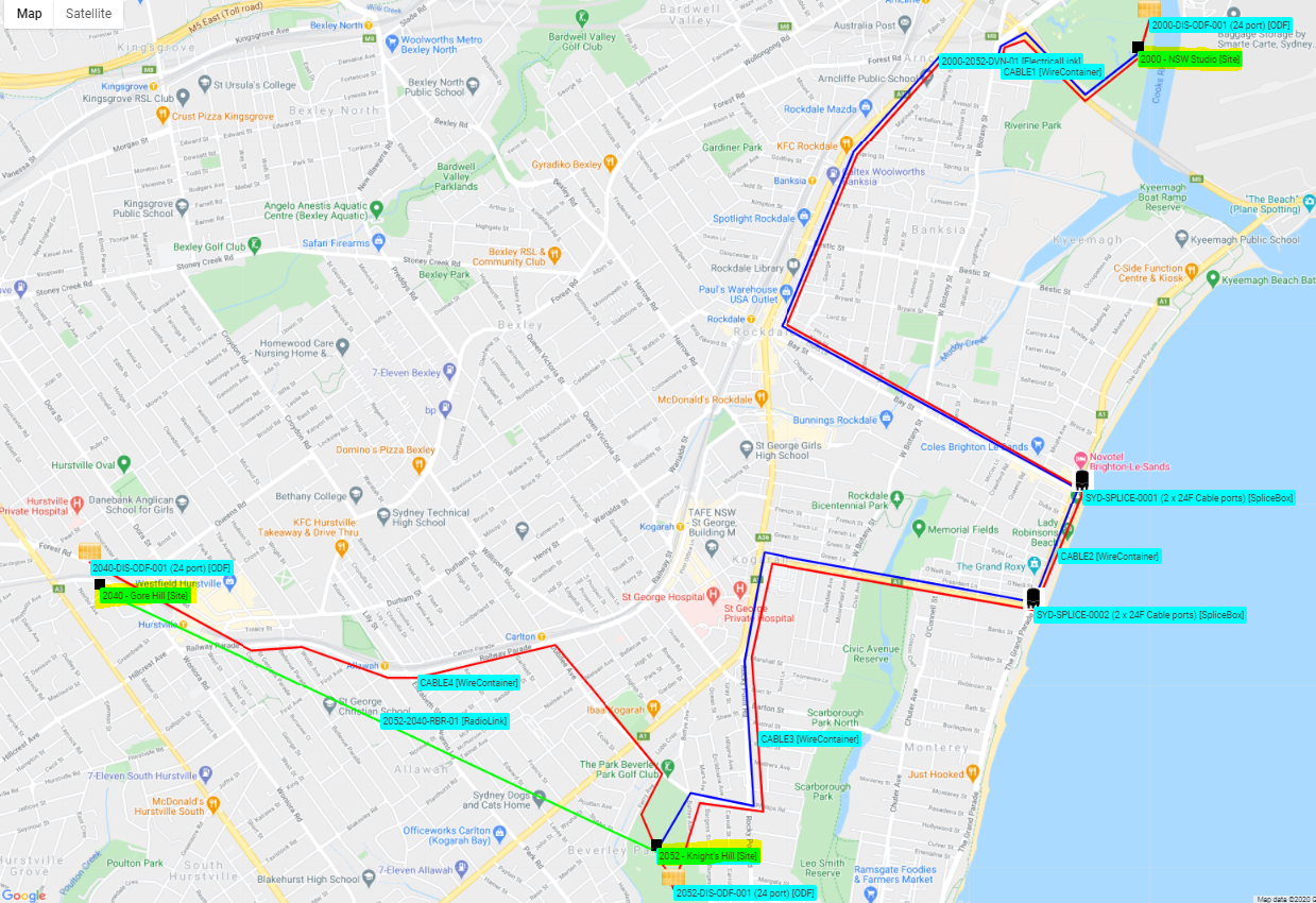
You may also have noticed that the green line is showing a radio broadcast link, which is point-to-point radio and therefore follows a straight line path from antenna to antenna.

Cable Management

Cable management and splicing / connections is supported, with tubes/strands being selected and then terminated at each end of the cable (in this case CABLE1 and its strands connect the splice case on the left pane, with the ODF on the right pane). These can be managed on a strand-by-strand basis via the central pane. From the diagram, we can see that fibre 001 in CABLE 1 is connected to F1-001 in the splice case and 001-back on the ODF from the A-end and B-end details in the bottom left corner.

From the naming convention, you’ll notice that there are two sets of cable “ports” in the splice case, as indicated by fibre numbers starting with F1 and F2 respectively.

Topology Views

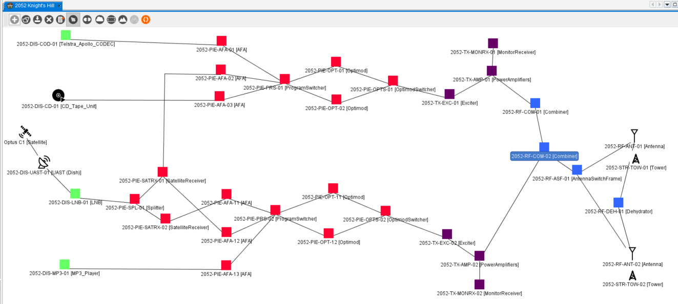
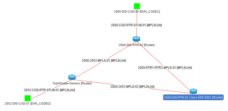
The diagram below shows a topological view of the devices within a site, helping operators to visualise connectivity relationships.

Services

One of the most important roles that inventory solutions play is as a repository of equipment and capacity. They also assist in allocating available resources to customer services. In the example below, service number “2052-ABC_LR_97.3FM-BSO” has a dependency on a tower, antenna, antenna switch frame and many more devices. If any of these devices fails, it will impact this customer service, as we’ll describe in more detail below.

IP Address Management (IPAM) and IP Assignment

We can manage IP address ranges / subnets, such as the examples below:

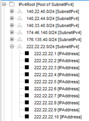
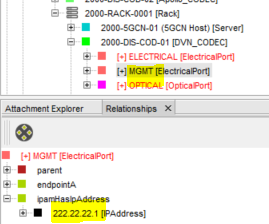
And then allocate individual IP addresses to devices, such as assigning IP address 222.22.22.1 to the CODEC, as shown on the “Physical Connection” diagram above.

MPLS Network

The following provides a simple MPLS network cloud for a customer:

APIs (including Service Impact Analysis Query)

The solution has hundreds of in-built APIs that facilitate queries, adds, modifies and deletes of data. 

The example shown below is getAffectedServices, which performs a service impact analysis. In this case, if we know that the device TEST-CD-02 fails, it will affect service number “2052-ABC_LR_97.3FM-BSO.” We can also look up the attributes of that service, which could include customer and customer contact details so that we can inform them their service is degraded and that repair processes have been initiated.

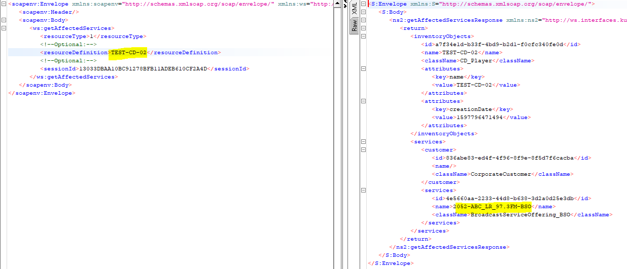
Note that the left-side pane is the Request and the right-side pane is the Response across the getAffectedServices API.

Data management via queries of the Graph Database

This inventory tool uses a Neo4j graph database. Using Neo4j browser, we can connect to the database and issue cypher queries (which are analogous to SQL, a structured query language that allows you to read/write data from/to the database). 

The screenshot below shows the constellation of linked data returned after issuing the cypher query (MATCH (n:InventoryObjects…. etc)). The data can also be exported in other formats, not just the graphical form shown here. 

I hope you enjoyed the brief introduction to the Inventory module of our Personal OSS Sandpit Project. Click on the link to step back to the parent page and see what other modules and/or use-cases are available for review.